Welcome to linvpy’s documentation !¶

LinvPy is a Python package designed to solve linear inverse problems of the form :

\[y = Ax + n\]

where $y$ is a vector of measured values, $A$ is a known matrix, $x$ is an unknown input vector and $n$ is noise.

The goal is to find $x$, or at least the best possible estimation; if the matrix $A$ is invertible, the solution is easy to find by multiplying by the inverse, if not, we need to use regression techniques such as least squares method to find $x$. The first motivation for this project is that Marta Martinez-Camara, PhD student in Communications Systems at EPFL (Switzerland) designed some new algorithms for solving linear inverse problems. LinvPy is a Python implementation of these algorithms, which may not be available anywhere else than here. LinvPy also contains several other known functions such as loss functions regularization functions or M-estimators.

Source code is on GitHub : https://github.com/LCAV/linvpy.

Paper of reference: The regularized tau estimator: A robust and efficient solution to ill-posed linear inverse problems, by Martinez-Camara et al. You can find it at: https://arxiv.org/abs/1606.00812

Get it¶

LinvPy is available from PyPi and Python 2.7 compatible. If you have pip already installed, simply run :

$ sudo pip2 install --ignore-installed --upgrade linvpy

If you don’t have pip installed, run :

$ sudo easy_install pip
$ sudo pip2 install --ignore-installed --upgrade linvpy

Quick start¶

To solve $y=Ax$ with outliers knowing $y, A$ :

import numpy as np
import linvpy as lp

a = np.matrix([[1, 2], [3, 4], [5, 6]])
y = np.array([1, 2, 3])

You can create a tau estimator object with the default parameters :

# Using the Tau-estimator :
tau = lp.TauEstimator()
tau.estimate(a,y)
# returns : (array([  1.45956448e-16,   5.00000000e-01]), 1.9242827743815571)
# where array([  1.45956448e-16,   5.00000000e-01]) is the best x to solve y=Ax
# and 1.9242827743815571 is the value of the tau scale for this x

Or an M estimator :

# Using the M-estimator :
m = lp.MEstimator()
m.estimate(a,y)
# returns [ -2.95552481e-16   5.00000000e-01], the best x to solve y=Ax

You can easily choose the loss function you want to use when you create the object :

# By default both estimators use the Huber loss function, but you can use any of Huber, Cauchy, Bisquare or Optimal (all described in the doc below) :
tau = lp.TauEstimator(loss_function=lp.Cauchy)
tau.estimate(a,y)

And the rest of the parameters:

# or you can give one, two, three... or all parameters :
tau = lp.TauEstimator(
    loss_function=lp.Optimal,
    clipping_1=0.6,
    clipping_2=1.5,
    lamb=3,
    scale=1.5,
    b=0.7,
    tolerance=1e4, )
tau.estimate(a,y)

Or you can change the parameters later:

# to change the clipping or any other parameter of the estimator :
tau.loss_function_1.clipping = 0.7
tau.tolerance = 1e3
m.lamb = 3

You can also choose a particular initial solution for the irls algorithm. To get the solution you run the method ‘estimate’ with your data a and y, and initial solution x_0 if any (this is not necessary):

# running with an initial solution :
x = np.array([5, 6])
x_tau_estimate = tau.estimate(a,y, initial_x=x)
m_tau_estimate = m.estimate(a,y, initial_x=x)

Module contents¶

Estimators

`MEstimator`	The M-estimator uses the method of iteratively reweighted least squares (IRLS) to minimize iteratively the function:
`TauEstimator`	Description of the tau-estimator

Loss Functions

Bisquare

param clipping:	Value of the clipping to be used in the loss function

Cauchy

param clipping:	Value of the clipping to be used in the loss function

Huber

param clipping:	Value of the clipping to be used in the loss function

Optimal

param clipping:	Value of the clipping to be used in the loss function

Regularization Functions

`Lasso`	Lasso algorithm that solves $min \|\|\mathbf{y - Ax}\|\|_2^2 + lambda \|\|x\|\|_1$
`Tikhonov`	The standard approach to solve the problem $\mathbf{y = Ax + n}$ explained above is to use the ordinary least squares method.

Using custom regularization functions¶

To use a custom regularization function :

copy paste this code into your python file
change the name CustomRegularization with the name of your function
define the regularization function in the definition of regularize
create your custom tau by passing an instance of your regularization, i.e. with “()” after the name

# Define your own regularization that extends lp.Regularization
class CustomRegularization(lp.Regularization):
    pass
    # Define your regularization function here
    def regularize(self, a, y, lamb=0):
        return np.ones(a.shape[1])

a = np.matrix([[1, 2], [3, 4], [5, 6]])
y = np.array([1, 2, 3])

# Create your custom tau estimator with custom regularization function
# Pay attention to pass the loss function as a REFERENCE (without the "()"
# after the name, and the regularization as an OBJECT, i.e. with the "()").
custom_tau = lp.TauEstimator(regularization=CustomRegularization())
print custom_tau.estimate(a,y)

Using custom loss functions¶

To use a custom loss function :

copy paste this code into your python file
change the name “CustomLoss” with the name of your loss function
change the two “0.7” with the value of your default clipping
define your rho function in the unit_rho definition
define your psi function as the derivative of the rho function in unit_psi
create your own tau estimator by passing your loss function name to it

# Define your own loss function that extends lp.LossFunction
class CustomLoss(lp.LossFunction):

    # Set your custom clipping
    def __init__(self, clipping=0.7):
        lp.LossFunction.__init__(self, clipping)
        if clipping is None:
            self.clipping = 0.7

    # Define your rho function : you can copy paste this and just change what's
    # inside the unit_rho
    def rho(self, array):
        # rho function of your loss function on ONE single element
        def unit_rho(element):
            # Simply return clipping * element for example
            return element + self.clipping
        # Vectorize the function
        vfunc = np.vectorize(unit_rho)
        return vfunc(array)

    # Define your psi function as the derivative of the rho function : you can
    # copy paste this and just change what's inside the unit_psi
    def psi(self, array):
        # rho function of your loss function on ONE single element
        def unit_psi(element):
            # Simply return the clipping for example
            return 1
        # Vectorize the function
        vfunc = np.vectorize(unit_psi)
        return vfunc(array)

a = np.matrix([[1, 2], [3, 4], [5, 6]])
y = np.array([1, 2, 3])

custom_tau = lp.TauEstimator(loss_function=CustomLoss)
print custom_tau.estimate(a,y)

Tutorial¶

Why do we need robust estimators?¶

The nature of the errors that appear in a problem may pose a significant challenge. This is quite an old problem, and it was already mentioned in the first publications about least squares, more than two centuries ago. Legendre wrote in 1805

If among these errors are some which appear too large to be admissible, then those observations which produced these errors will be rejected, as coming from too faulty experiments, and the unknowns will be determined by means of the other observations, which will then give much smaller errors.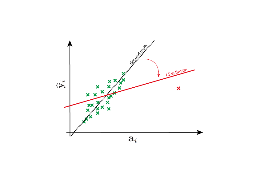

Contribute¶

If you want to contribute to this project, feel free to fork our GitHub main repository repository : https://github.com/LCAV/linvpy. Then, submit a ‘pull request’. Please follow this workflow, step by step:

Fork the project repository: click on the ‘Fork’ button near the top of the page. This creates a copy of the repository in your GitHub account.
Clone this copy of the repository in your local disk.
Create a branch to develop the new feature :
```
$ git checkout -b new_feature
```

Work in this branch, never in the master branch.

To upload your changes to the repository :

$ git add modified_files
$ git commit -m "what did you implement in this commit"
$ git push origin new_feature

When your are done, go to the webpage of the main repository, and click ‘Pull request’ to send your changes for review.

Documentation¶

class linvpy.Bisquare(clipping=4.685)[source]¶

Bases: linvpy.LossFunction

Parameters:	clipping (float) – Value of the clipping to be used in the loss function

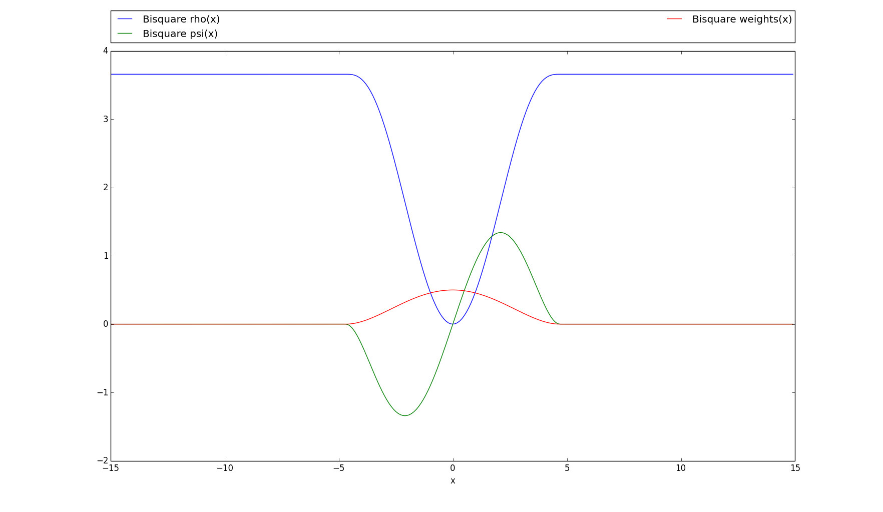
psi(array)[source]¶

The derivative of bisquare loss (or Tukey’s loss), “psi” version.

$\psi(x)=\begin{cases} x((1-(\frac{x}{c})^2)^2)& \text{if |x|} \leq c \\ 0& \text{if |x| > c} \end{cases}$

Parameters:	array (numpy.ndarray) – Array of values to apply the loss function to
Returns:	Array of same shape as the input, cell-wise results of the loss function
Return type:	numpy.ndarray
Example:

>>> import numpy as np
>>> import linvpy as lp

>>> bisquare = lp.Bisquare()
>>> bisquare.psi(2)
array(1.3374668237772656)

>>> y = np.array([1, 2, 3])
>>> bisquare.psi(y)
array([ 0.9109563 ,  1.33746682,  1.04416812])

>>> a = np.matrix([[1, 2], [3, 4], [5, 6]])
>>> bisquare.psi(a)
matrix([[ 0.9109563 ,  1.33746682],
    [ 1.04416812,  0.2938613 ],
    [ 0.        ,  0.        ]])

rho(array)[source]¶

The regular bisquare loss (or Tukey’s loss), “rho” version.

$\rho(x)=\begin{cases} (\frac{c^2}{6})(1-(1-(\frac{x}{c})^2)^3)& \text{if |x|} \leq 0 \\ \frac{c^2}{6}& \text{if |x| > 0} \end{cases}$

Parameters:	array (numpy.ndarray) – Array of values to apply the loss function to
Returns:	Array of same shape as the input, cell-wise results of the loss function
Return type:	numpy.ndarray
Example:

>>> import numpy as np
>>> import linvpy as lp

>>> bisquare = lp.Bisquare()
>>> bisquare.rho(2)
array(1.6576630874988754)

>>> y = np.array([1, 2, 3])
>>> bisquare.rho(y)
array([ 0.4775661 ,  1.65766309,  2.90702817])

>>> a = np.matrix([[1, 2], [3, 4], [5, 6]])
>>> bisquare.rho(a)
matrix([[ 0.4775661 ,  1.65766309],
    [ 2.90702817,  3.58536054],
    [ 3.65820417,  3.65820417]])

>>> # Plots the rho, psi and m_weights on the given interval
>>> bisquare.plot(15)

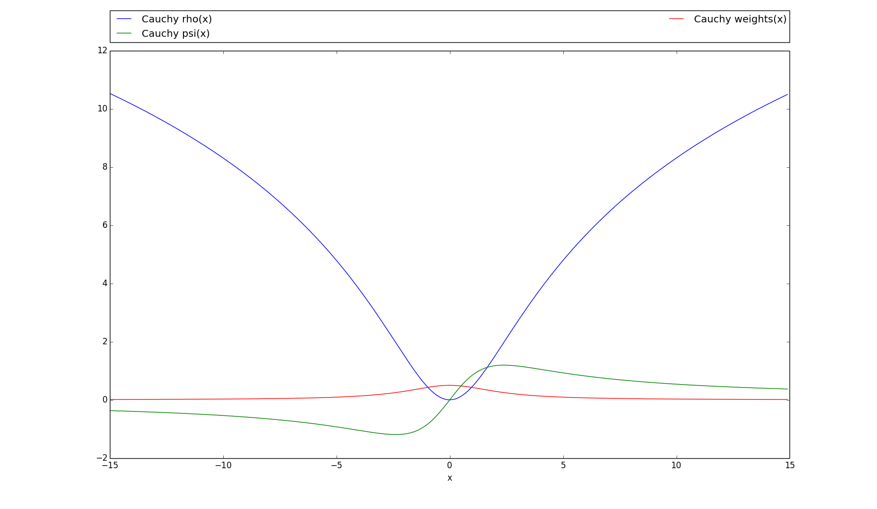
class linvpy.Cauchy(clipping=2.3849)[source]¶

Bases: linvpy.LossFunction

Parameters:	clipping (float) – Value of the clipping to be used in the loss function

psi(array)[source]¶

Parameters:	array (numpy.ndarray) – Array of values to apply the loss function to
Returns:	Array of same shape as the input, cell-wise results of the loss function
Return type:	numpy.ndarray
Example:

>>> import numpy as np
>>> import linvpy as lp

>>> cauchy = lp.Cauchy()
>>> cauchy.psi(2)
array(1.1742146893434733)

>>> y = np.array([1, 2, 3])
>>> cauchy.psi(y)
array([ 0.85047284,  1.17421469,  1.16173317])

>>> a = np.matrix([[1, 2], [3, 4], [5, 6]])
>>> cauchy.psi(a)
matrix([[ 0.85047284,  1.17421469],
    [ 1.16173317,  1.0490251 ],
    [ 0.92671316,  0.81862153]])

rho(array)[source]¶

Parameters:	array (numpy.ndarray) – Array of values to apply the loss function to
Returns:	Array of same shape as the input, cell-wise results of the loss function
Return type:	numpy.ndarray
Example:

>>> import numpy as np
>>> import linvpy as lp

>>> cauchy = lp.Cauchy()
>>> cauchy.rho(2)
array(1.5144982928548816)

>>> y = np.array([1, 2, 3])
>>> cauchy.rho(y)
array([ 0.46060182,  1.51449829,  2.69798124])

>>> a = np.matrix([[1, 2], [3, 4], [5, 6]])
>>> cauchy.rho(a)
matrix([[ 0.46060182,  1.51449829],
    [ 2.69798124,  3.80633511],
    [ 4.79348926,  5.66469239]])

>>> # Plots the rho, psi and m_weights on the given interval
>>> cauchy.plot(15)

class linvpy.Huber(clipping=1.345)[source]¶

Bases: linvpy.LossFunction

Parameters:	clipping (float) – Value of the clipping to be used in the loss function

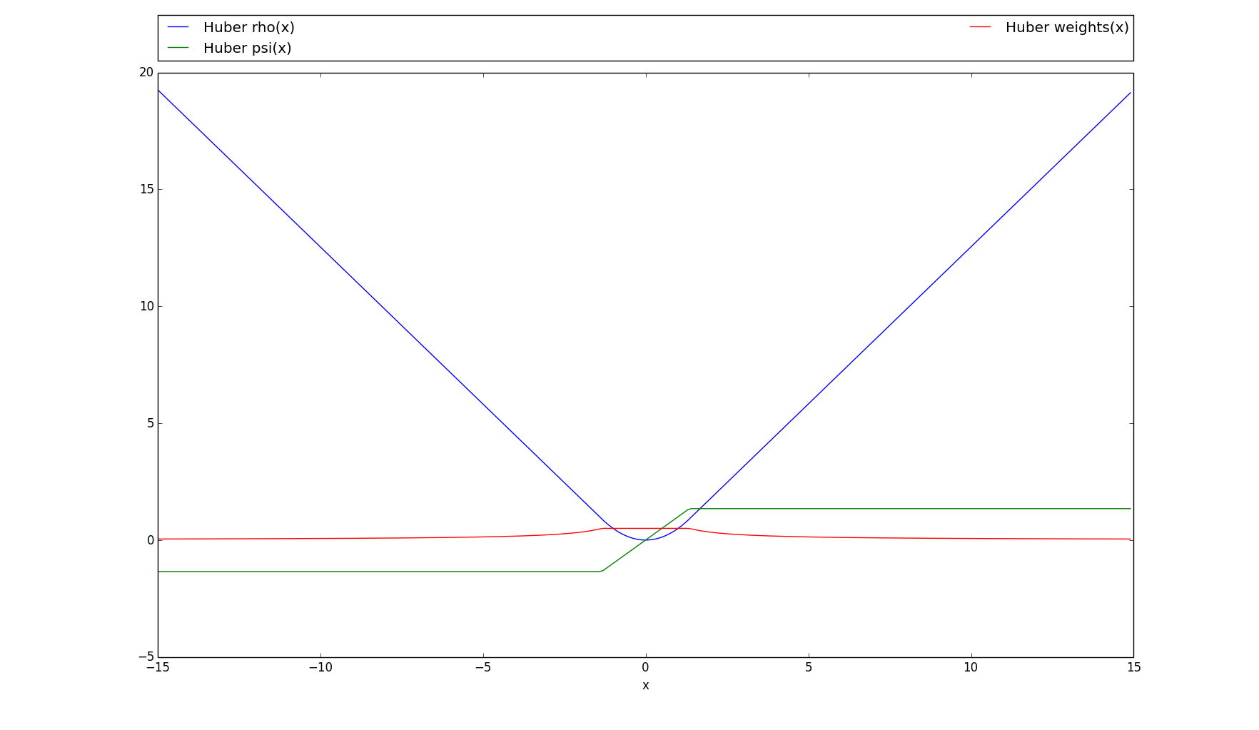
psi(array)[source]¶

Derivative of the Huber loss function; the “psi” version. Used in the weight function of the M-estimator.

$\psi(x)=\begin{cases} x& \text{if |x|} \leq clipping \\ clipping \cdot sign(x) & \text{otherwise} \end{cases}$

Parameters:	array (numpy.ndarray) – Array of values to apply the loss function to
Returns:	Array of same shape as the input, cell-wise results of the loss function
Return type:	numpy.ndarray
Example:

>>> import numpy as np
>>> import linvpy as lp

>>> huber = lp.Huber()
>>> huber.psi(2)
array(1.345)

>>> y = np.array([1, 2, 3])
>>> huber.psi(y)
array([ 1.   ,  1.345,  1.345])

>>> a = np.matrix([[1, 2], [3, 4], [5, 6]])
>>> huber.psi(a)
matrix([[ 1.   ,  1.345],
    [ 1.345,  1.345],
    [ 1.345,  1.345]])

rho(array)[source]¶

The regular huber loss function; the “rho” version.

$\rho(x)=\begin{cases} \frac{1}{2}{x^2}& \text{if |x|} \leq clipping \\ clipping (|x| - \dfrac{1}{2} clipping)& \text{otherwise} \end{cases}$

This function is quadratic for small inputs, and linear for large inputs.

Parameters:	array (numpy.ndarray) – Array of values to apply the loss function to
Returns:	Array of same shape as the input, cell-wise results of the loss function
Return type:	numpy.ndarray
Example:

>>> import numpy as np
>>> import linvpy as lp

>>> huber = lp.Huber()
>>> huber.rho(2)
array(1.7854875000000001)

>>> y = np.array([1, 2, 3])
>>> huber.rho(y)
array([ 0.5      ,  1.7854875,  3.1304875])

>>> a = np.matrix([[1, 2], [3, 4], [5, 6]])
>>> huber.rho(a)
matrix([[ 0.5      ,  1.7854875],
    [ 3.1304875,  4.4754875],
    [ 5.8204875,  7.1654875]])

>>> # Plots the rho, psi and m_weights on the given interval
>>> huber.plot(15)

class linvpy.Lasso[source]¶

Bases: linvpy.Regularization

Lasso algorithm that solves $min ||\mathbf{y - Ax}||_2^2 + lambda ||x||_1$

regularize(a, y, lamb=0)[source]¶

Parameters:	a (numpy.ndarray) – MxN matrix A in the y=Ax equation y (numpy.ndarray) – M vector y in the y=Ax equation lamb (integer) – non-negative regularization parameter
Returns:	N vector x in the y=Ax equation
Return type:	numpy.ndarray
Example:

>>> import numpy as np
>>> import linvpy as lp

>>> a = np.matrix([[1, 2], [3, 4], [5, 6]])
>>> y = np.array([1, 2, 3])

>>> lasso = lp.Lasso()

>>> lasso.regularize(a, y, 2)
array([ 0.        ,  0.48214286])

>>> lasso.regularize(a, y)
array([ -5.97106181e-17,   5.00000000e-01])

class linvpy.MEstimator(loss_function=<class linvpy.Huber>, clipping=None, regularization=<linvpy.Tikhonov instance>, lamb=0, scale=1.0, b=0.5, tolerance=1e-05, max_iterations=100)[source]¶

Bases: linvpy.Estimator

The M-estimator uses the method of iteratively reweighted least squares (IRLS) to minimize iteratively the function:

$\boldsymbol x^{(t+1)} =$ ${\rm arg}\min_x\,$ $\big|\big| \boldsymbol W (\boldsymbol x^{(t)})(\boldsymbol y - \boldsymbol A \boldsymbol x )\big | \big |_2^2.$

The IRLS is used, among other things, to compute the M-estimate and the tau-estimate.

Parameters:

Parameters:	loss_function (linvpy.LossFunction type) – loss function to be used in the estimation clipping (float) – clipping to be used in the loss function regularization (linvpy.Regularization type) – regularization function to regularize the y=Ax system lamb (integer) – lambda to be used in the regularization (lambda = 0 is equivalent to using least squares) scale (float) – b (float) – tolerance (float) – treshold : when residuals < tolerance, the current solution is returned max_iterations (integer) – maximum number of iterations of the iteratively reweighted least squares

loss_function (linvpy.LossFunction type) – loss function to be used in the estimation
clipping (float) – clipping to be used in the loss function
regularization (linvpy.Regularization type) – regularization function to regularize the y=Ax system
lamb (integer) – lambda to be used in the regularization (lambda = 0 is equivalent to using least squares)
scale (float) –
b (float) –
tolerance (float) – treshold : when residuals < tolerance, the current solution is returned
max_iterations (integer) – maximum number of iterations of the iteratively reweighted least squares

estimate(a, y, initial_x=None)[source]¶

Parameters:	a (numpy.ndarray) – MxN matrix A in the y=Ax equation y (numpy.ndarray) – M vector y in the y=Ax equation initial_x (numpy.ndarray) – N vector of an initial solution
Returns:	best estimation of the N vector x in the y=Ax equation
Return type:	numpy.ndarray
Example:

>>> import numpy as np
>>> import linvpy as lp

>>> a = np.matrix([[1, 2], [3, 4], [5, 6]])
>>> y = np.array([1, 2, 3])

>>> m = lp.MEstimator()
>>> m.estimate(a,y)
array([ -2.95552481e-16,   5.00000000e-01])

>>> m_ = lp.MEstimator(loss_function=lp.Bisquare, clipping=2.23,         regularization=lp.Lasso(), lamb=3)
>>> initial_solution = np.array([1, 2])
>>> m_.estimate(a, y, initial_x=initial_solution)
array([ 0.,  0.])

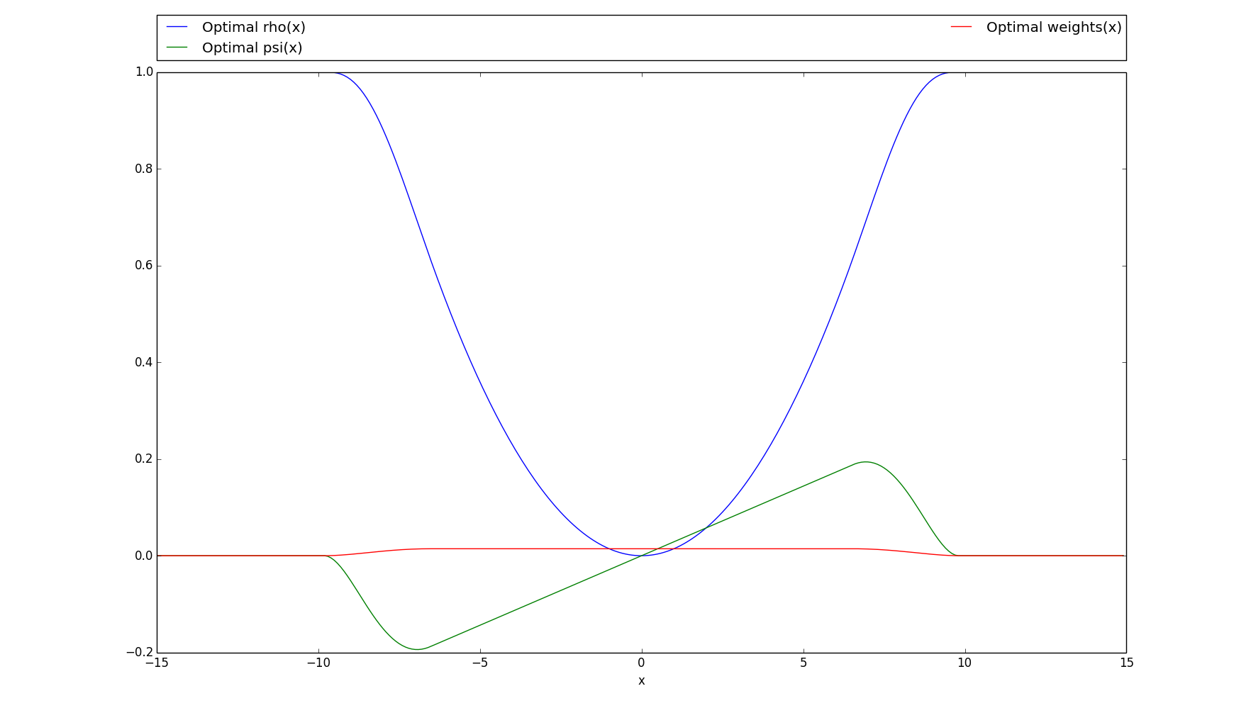
class linvpy.Optimal(clipping=3.27)[source]¶

Bases: linvpy.LossFunction

Parameters:	clipping (float) – Value of the clipping to be used in the loss function

psi(array)[source]¶

Parameters:	array (numpy.ndarray) – Array of values to apply the loss function to
Returns:	Array of same shape as the input, cell-wise results of the loss function
Return type:	numpy.ndarray
Example:

>>> import numpy as np
>>> import linvpy as lp

>>> optimal = lp.Optimal()
>>> optimal.psi(2)
array(0.05755076877036309)

>>> y = np.array([1, 2, 3])
>>> optimal.psi(y)
array([ 0.02877538,  0.05755077,  0.08632615])

>>> a = np.matrix([[1, 2], [3, 4], [5, 6]])
>>> optimal.psi(a)
matrix([[ 0.02877538,  0.05755077],
    [ 0.08632615,  0.11510154],
    [ 0.14387692,  0.17265231]])

rho(array)[source]¶

Parameters:	array (numpy.ndarray) – Array of values to apply the loss function to
Returns:	Array of same shape as the input, cell-wise results of the loss function
Return type:	numpy.ndarray
Example:

>>> import numpy as np
>>> import linvpy as lp

>>> optimal = lp.Optimal()
>>> optimal.rho(2)
array(0.057550768770363074)

>>> y = np.array([1, 2, 3])
>>> optimal.rho(y)
array([ 0.01438769,  0.05755077,  0.12948923])

>>> a = np.matrix([[1, 2], [3, 4], [5, 6]])
>>> optimal.rho(a)
matrix([[ 0.01438769,  0.05755077],
    [ 0.12948923,  0.23020308],
    [ 0.3596923 ,  0.51795692]])

>>> # Plots the rho, psi and m_weights on the given interval
>>> optimal.plot(15)

class linvpy.TauEstimator(loss_function=<class linvpy.Huber>, clipping_1=None, clipping_2=None, regularization=<linvpy.Tikhonov instance>, lamb=0, scale=1.0, b=0.5, tolerance=1e-05, max_iterations=100)[source]¶

Bases: linvpy.Estimator

Description of the tau-estimator

Parameters:

Parameters:	loss_function (linvpy.LossFunction type) – loss function to be used in the estimation clipping_1 (float) – first clipping value of the loss function clipping_2 (float) – second clipping value of the loss function regularization (linvpy.Regularization type) – regularization function to regularize the y=Ax system lamb (integer) – lambda to be used in the regularization (lambda = 0 is equivalent to using least squares) scale (float) – b (float) – tolerance (float) – treshold : when residuals < tolerance, the current solution is returned max_iterations (integer) – maximum number of iterations of the iteratively reweighted least squares

loss_function (linvpy.LossFunction type) – loss function to be used in the estimation
clipping_1 (float) – first clipping value of the loss function
clipping_2 (float) – second clipping value of the loss function
regularization (linvpy.Regularization type) – regularization function to regularize the y=Ax system
lamb (integer) – lambda to be used in the regularization (lambda = 0 is equivalent to using least squares)
scale (float) –
b (float) –
tolerance (float) – treshold : when residuals < tolerance, the current solution is returned
max_iterations (integer) – maximum number of iterations of the iteratively reweighted least squares

estimate(a, y, initial_x=None)[source]¶

This routine minimizes the objective function associated with the tau-estimator. For more information on the tau estimator see http://arxiv.org/abs/1606.00812

This function is hard to minimize because it is non-convex. This means that it has several local minimums; depending on the initial x that is used, the algorithm ends up in a different local minimum.

This algorithm takes the ‘brute force’ approach: it tries many different initial solutions, and picks the minimum with smallest value. The output of this estimation is the best minimum found.

Return x_hat, tscalesquare:
Parameters:	a (numpy.ndarray) – MxN matrix A in the y=Ax equation y (numpy.ndarray) – M vector y in the y=Ax equation initial_x (numpy.ndarray) – N vector of an initial solution
	best estimation of the N vector x in the y=Ax equation and value of the tau scale
Return type:	Tuple[numpy.ndarray, numpy.float64]
Example:

>>> import numpy as np
>>> import linvpy as lp

>>> a = np.matrix([[1, 2], [3, 4], [5, 6]])
>>> y = np.array([1, 2, 3])

>>> tau = lp.TauEstimator()
>>> tau.estimate(a,y)
(array([  1.45956448e-16,   5.00000000e-01]), 1.9242827743815571)

>>> tau_ = lp.TauEstimator(loss_function=lp.Cauchy, clipping_1=2.23,         clipping_2=0.7, regularization=lp.Lasso(), lamb=2)
>>> initial_solution = np.array([1, 2])
>>> tau_.estimate(a, y, initial_x=initial_solution)
(array([ 0.        ,  0.26464687]), 0.99364206111683273)

fast_estimate(a, y, initial_x=None, initial_iter=5)[source]¶

Fast version of the basic tau algorithm. To save some computational cost, this algorithm exploits the speed of convergence of the basic algorithm. It has two steps: in the first one, for every initial solution, it only performs initialiter iterations. It keeps value of the objective function. In the second step, it compares the value of all the objective functions, and it select the nmin smaller ones. It iterates them until convergence. Finally, the algorithm select the x that produces the smallest objective function. For more details see http://arxiv.org/abs/1606.00812

Return x_hat, tscalesquare:
Parameters:	a (numpy.ndarray) – MxN matrix A in the y=Ax equation y (numpy.ndarray) – M vector y in the y=Ax equation initial_x (numpy.ndarray) – N vector of an initial solution initial_iter (integer) – number of iterations to be performed
	best estimation of the N vector x in the y=Ax equation and value of the tau scale
Return type:	Tuple[numpy.ndarray, numpy.float64]
Example:

>>> import numpy as np
>>> import linvpy as lp

>>> a = np.matrix([[1, 2], [3, 4], [5, 6]])
>>> y = np.array([1, 2, 3])

>>> tau = lp.TauEstimator()
>>> tau.fast_estimate(a,y)
(array([  1.45956448e-16,   5.00000000e-01]), 1.9242827743815571)

>>> tau_ = lp.TauEstimator(loss_function=lp.Cauchy, clipping_1=2.23,         clipping_2=0.7, regularization=lp.Lasso(), lamb=2)
>>> initial_solution = np.array([1, 2])
>>> tau_.fast_estimate(a, y, initial_x=initial_solution,         initial_iter=6)
(array([ 0.        ,  0.26464805]), 0.99363748192798829)

class linvpy.Tikhonov[source]¶

Bases: linvpy.Regularization

The standard approach to solve the problem $\mathbf{y = Ax + n}$ explained above is to use the ordinary least squares method. However if your matrix $\mathbf{A}$ is a fat matrix (it has more columns than rows) or it has a large condition number, then you should use a regularization to your problem in order to get a meaningful estimation of $\mathbf{x}$.

The Tikhonov regularization is a tradeoff between the least squares solution and the minimization of the L2-norm of the output $x$ ( L2-norm = sum of squared values of the vector $x$), $\hat{ \mathbf{x}} = {\rm arg}\min_x\,\lVert \mathbf{y - Ax} \rVert_2^2 + \lambda\lVert \mathbf{x} \rVert_2^2$

The parameter lambda tells how close to the least squares solution the output $\mathbf{x}$ will be; a large lambda will make $\mathbf{x}$ close to $\lVert\mathbf{x}\rVert_2^2 = 0$, while a small lambda will approach the least squares solution (Running the function with lambda=0 will behave like the ordinary least_squares() method).

The Tikhonov solution has an analytic solution and it is given by $\hat{\mathbf{x}} = (\mathbf{A^{T}A}+ \lambda^{2} \mathbf{ I})^{-1}\mathbf{A}^{T}\mathbf{y}$, where $\mathbf{I}$ is the identity matrix.

regularize(a, y, lamb=0)[source]¶

Parameters:	a (numpy.ndarray) – MxN matrix A in the y=Ax equation y (numpy.ndarray) – M vector y in the y=Ax equation lamb (integer) – non-negative tradeoff parameter between least squares and minimization of the L-2 norm
Returns:	N vector x in the y=Ax equation
Return type:	numpy.ndarray
Example:

>>> import numpy as np
>>> import linvpy as lp

>>> a = np.matrix([[1, 2], [3, 4], [5, 6]])
>>> y = np.array([1, 2, 3])

>>> tiko = lp.Tikhonov()

>>> tiko.regularize(a, y, 2)
array([ 0.21782178,  0.30693069])

>>> tiko.regularize(a, y)
array([ -5.97106181e-17,   5.00000000e-01])

Indices and tables¶

Index Module Index Search Page

`Lasso`	Lasso algorithm that solves \(min \|\|\mathbf{y - Ax}\|\|_2^2 + lambda \|\|x\|\|_1\)
`Tikhonov`	The standard approach to solve the problem \(\mathbf{y = Ax + n}\) explained above is to use the ordinary least squares method.